I am working on a baseball video game with 3D characters. Sometimes the characters need to move and they need to get to specific locations at specific times. But that’s tricky to do.
The problem is that the character runs via animation. Similar to how humans run, forward speed changes throughout the character’s running stride. Unlike how humans run though, animation is choppy. Each frame of the animation jumps from one position to the next. This choppiness can also be frame-rate dependent. Depending on the frame rate, animations can be interpolated differently, yielding slightly different forward speeds.
Additionally, the animation will also yield different forward speeds for different characters. Characters with longer legs will move faster for the same animation than characters with shorter legs.
The forward speed controls when we arrive at our target. And we can control the forward speed by controlling the animation speed. But because of the non-uniform speed through a stride, the frame-dependent interpolation, and the character dependence, the animation speed is a noisy controller for the forward speed. Making a 10% change in the animation speed may not necessarily yield a 10% change in the forward speed.
So how can we use our noisy control (animation speed) to finely control the arrival time of the character?
Proportional Control
The first step we can take is to add a proportional control. We check our current trajectory
and see if we will arrive early or late. If we are going to arrive early,
we can slow down by some factor. If we are going to arrive late, then we can
speed up by some factor. Let’s call the proportional factor P.
current_error = target_value - current_value
adjustment = P*current_error

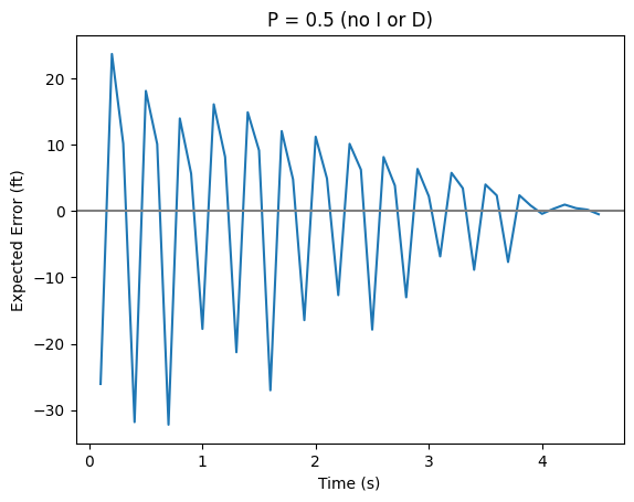
One problem here is how should we pick the factor. If the factor is too small, then we will be too slow to adjust. If the factor is too big, then we will overshoot.
Worse, the factor has to be different for different characters. As we established earlier, different characters are affected by the animation differently. And different adjustments to the animation speed will impact different characters differently as well.
So ideally we want to pick a “close enough” factor and have something else clean
up the edge cases for us. That’s where the I term comes in.
Integral Control
Suppose you picked a proportional factor that’s too low and the controls are not making adjustments fast enough. We can try to detect this situation and automatically push the adjustment in the needed direction.
For example, we can track the historical error by accumulating the error at each
measurement. We can use the accumulated error and adjust the speed by
another factor. As the accumulated error grows, we make a more aggressive adjustment.
Since the accumulated error can be seen as an integral, we can
call this factor the integral factor (or I).
historical_error += current_error
adjustment = P*current_error + I*historical_error

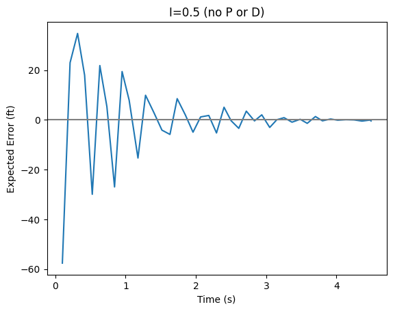
When we add the proportional and the integral controls, what we will see is that the integral factor will help the controller make faster adjustments but it will always overshoot the target. Since the accumulated error will not clear out till you start accumulating error in the other direction, the integral factor will always push you to go past the target to accumulate more error.
That’s where the D term can help us.
Derivative Control
The only remaining problem is to deal with the overshoot. To prevent overshoot, we can start by predicting the overshoot. We can look at the current change in error and use that to predict what the next error term will be. We can do that just by looking at the difference between the previous and current error and assuming that the same change will happen again (this is kinda like approximating the derivative).
If we see that we are going to overshoot, we can add yet one more scaling
factor to resist the overshoot. We can call this factor the “derivative” factor (or D).
We use the time between the current measurement and the previous measurement as dt.
future_error = (current_error - prev_error)/dt
adjustment = P*current_error
         + I*historical_error
         + D*future_error
Using PIDs
At this point, we have fully derived PID controllers. PID controllers combine historical behavior, current error, and future prediction to adjust the controls of a system. PIDs help you figure out adjustments needed to push a system to a desired state.
To use it though, we still have to decide how to actually use the adjustment
value and have to pick the values for P, I, and D.
Since the adjustment value will naturally be negative when the error is in one direction and positive in the other, it is useful to treat adjustment as a number that can be both. To simplify the handling of the adjustment, we can restrict the number to be between -1 and 1. Any scaling that needs to be done can be done by us.
So we can use the adjustment this way:
// normalized will be between 0 and 1
normalized = 0.5 + 0.5*adjustment
new_speed = max_speed*normalized
Since normalized will be between 0 and 1, new_speed will always be between 0 and max_speed.
Now we are in a place where we can start testing to pick the correct values for our factors.
For my use case, I found that the derivative term was very noisy. In real physical
systems, the derivatives are smoother but here
I was working with artificial animation that is not as smooth. So to keep the derivative term in check,
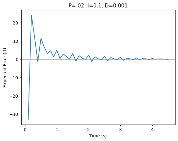
I set D to be very small - on the order of 1/1,000. So the D term would only come into play when there is severe overshoot.
I didn’t want any adjustment to be very sudden so I set P to be around 1/20 to 1/10. This basically
meant that the proportional reaction was limited to 5% to 10%. To
make sure that we did reach our target though, I set the I term to be around the same range of 1/10.
This meant that the animation made small adjustments and became more aggressive if the error accumulated.

In the end, I was able to get the animation to have the same accuracy as the frequency of my adjustments. I decided to make adjustments every 100ms–I didn’t want to make adjustments any more frequently to avoid jarring changes in the animation.
PIDs
PIDs are very commonly used in systems that need to adapt. This can be cruise control in cars that need to adjust power when going uphill, robots that need to react to a push, or industrial systems that need to adapt to the changing behavior of different subsystems.
Despite its apparent simplicity, PIDs weren’t formulated in this form till the early 1900s. They were designed to capture the intuition of sailors steering a ship–the sailors would steer accounting for the current error but would also account for past and future errors to make adjustments. I love how well PIDs capture that intuition.
When I faced my original problem, I vaguely knew that I wanted to make adjustments to the speed based on the current error but I could quickly come up with more and more edge cases that I would have to handle individually. This would have been a very brittle approach. PIDs allowed me to implement a much more flexible solution that is also simpler than what I would have done.
No wonder they are used so frequently.
Other Resources
- Vazgriz - PID Controllers in Unity3D is a beautiful blog post with visualizations of PIDs in action.
- Wikipedia highlights the more general use cases in industrial systems.