Electron At The End of The Universe
Physics gives us a deterministic model of the universe.1 Given the current state of a system, we can predict how the system will look at any future time.
If there is a ball moving left at 1m/s we can predict that in 2 seconds it will have moved 2 meters to the left. An assumption we are making here is that the only factor to consider is the ball’s velocity. But if the ball was moving on a rough surface, then the surface friction would be important to include in our calculation.
So the accuracy of our predictions depends on our ability to correctly decide what is and isn’t important to include in our system. How can we make this decision? If we don’t include the important things in our calculations (like surface friction), then our calculations will be wrong. However, if we decide that everything is important, then we can’t calculate anything because it would be impossible to measure ALL things in the universe.
Somehow, we have to find a line between what is important and what is negligible. To help us with our intuition, we will start with an extreme system.
The following instructive example is based on an essay by Michael Berry titled “The Electron at the End of the Universe”.
Let’s imagine that we are in a mostly empty universe. The universe has a 1m box at the center of it. The box is full of air. The only other thing in this universe is one tiny little electron, 13 billion light years away at the edge of the observable universe.
Now the question is: is the electron important or negligible to the movement of the air molecules in our box? I think the intuitive answer here is that it should be negligible. The electron is literally at the end of the universe! It would be like us having to worry about the exact position of the Curiosity rover on Mars for our day-to-day activities.
But let’s put our intuition to the test. Let’s imagine that we recorded each molecule’s starting position and velocity. We move each molecule according to their velocity and anytime two molecules collide, we update their trajectory based on the angle they collide at.
How wrong will our calculation be if we ignore the influence of the electron? Fortunately, we don’t have to do this calculation because the work is already done here and summarized here.
The error in the new trajectory after the first collision is:
$$\Delta \theta_1 \approx \frac {2Gm} {r \cdot d^3} \left( \frac \ell v \right)^2$$
Here are what the symbols represent2:
- $G$ is the gravity constant which is small
- $m$ is the mass of the molecules which is tiny
- $r$ is the radius of the molecules which is small
- $d$ is the distance to the electron which is astronomical
- $\ell$ is the average distance a molecule travels before a collision which is small
- $v$ is the velocity of the particles which is big
Almost all of these factors help make the final result small (small numerators and big denominators). Plugging in actual rough values gives us:
$$\Delta \theta_1 \approx \frac {2\cdot 10^{-11} \cdot 10^{-30}} { 10^{-10} \cdot 10^{26\cdot3}} \left( \frac {10^{-7}} {10^3} \right)^2 = 10^{-127}$$
Woo! That’s a tiny error.
But with each collision, this error will accumulate, right? So how many collisions will it take before the error is no longer negligible? If each collision added the same amount of error, then we would be in a pretty good situation. It would take $10^{127}$ collisions before we had significant errors and that many collisions haven’t even happened in the lifetime of our real universe.
Unfortunately, we are not so lucky. The errors here grow exponentially. The formula for the accumulated error on the Nth collision is:
$$ \Delta \theta_N = \left( \frac \ell r \right)^N \Delta \theta_1 = (10^3)^N \cdot 10^{-127}$$
Here is how quickly the error in the angle grows:
| N | Error $\Delta \theta_N$, radians |
|---|---|
| 1 | $10^{-127}$ |
| 10 | $10^{-100}$ |
| 20 | $10^{-70}$ |
| 30 | $10^{-40}$ |
| 40 | $10^{-10}$ |
| 50 | $10^{20}$ |
This means that somewhere in between 40 and 50 collisions, our predictions go from pretty good to completely useless because we failed to account for the gravitational pull of the electron. It would take our gas molecule a microsecond to experience 50 collisions. So within a microsecond, our system is overwhelmed by the tiny influence of the electron at the end of the universe!
Chaotic Systems

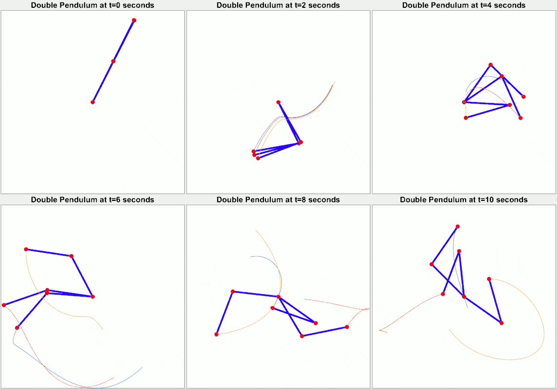
A system where small influences can result in large changes is known as a chaotic system. The commonly quoted example of a “butterfly flapping its wings and causing a hurricane” is an example of a chaotic system. But chaotic systems don’t even have to be all that complex. A double pendulum only has two moving parts but changing its starting position slightly will result in massively different trajectories.
Chaotic systems severely limit our ability to make predictions about them. We can’t measure the current state of the system perfectly. We can’t account for all possible influences on the system. So any predictions we make may be accurate for a short period but then errors will accumulate and the system will diverge quickly.
In school, we study systems with mostly linear relationships. But in reality, most real world systems have components with highly non-linear relationships. Most real world systems are chaotic.
For example, Hooke’s law says that the force on a spring is linearly proportional to how much it’s compressed. In reality, though, most materials have their own stress-strain curve that defines how that material responds to compression (and the curve is nonlinear). And this assumes even distribution of stress throughout the material, but in reality, stress will be unevenly applied throughout the material.

Living With Chaos
If chaotic systems are all around us and our predictions are useless, how exactly is the world still functioning? There are three main ways that we deal with chaos:
- Frequent Adjustments: The problem with our box of air was that we measured all the particles at the start and then let the errors accrue indefinitely. But if we remeasured often and adjusted our predictions, we would effectively be making short-term predictions which have lower errors. We use this strategy the most day-to-day. Every time we take a step, we predict where the ground will be, where our foot will be and our body readjusts based on new data mid-stride.
- Identifying Understood Regimes: A bridge can’t really remeasure its load and make frequent adjustments.3 When it’s built, it needs to be able to handle its job. The strategy here is to use materials that behave in well-understood ways in the capacity they will be used. For example, if the bridge uses a spring somewhere, then the spring should be made of a material that behaves in a well-understood way for the range of stress, temperature, and humidity the spring will have to face. Fortunately, the engineers don’t have to solve this problem all on their own. Manufacturers of all kinds of equipment and parts will publish the safe range of load for the different parts. So, spring manufacturers will document the regime where the spring follows Hooke’s law, resistor manufacturers will document the regime where the resistor follows Ohm’s law, and so on.
- Coarser Properties: In our prediction of each molecule, our errors grew exponentially. However, if we had instead predicted the temperature or pressure of the gas as a whole, our errors would have been much smaller. Temperature and pressure average out the noisiness of each molecule’s chaotic motion. The coarser properties have to be chosen properly though. Just because a property is coarser, it does not mean that it will filter out the chaos. The system has to be carefully studied to identify these coarser properties like the study of thermodynamics did for gases.
Long Term Predictions
The real-world is nonlinear. We mostly talked about physical systems but this applies even more to systems with people. Humans, individually and in groups, demonstrate path dependence, which means that their behavior depends on the history of the system. Systems with path dependence are highly nonlinear because minor historical events can have surprising effects later. So, for example, different humans will react differently when put in the same situation but all electrons will behave the same way no matter where the electrons have been before.
This is why, I think, we should be careful of making long term predictions.
Predictions for decades in the future are likely wrong. Predictions that define intermediate milestones provide a stronger base to evaluate the prediction on a rolling basis but the earlier milestones should be given more weight than the later milestones (like we do with weather predictions).
For example, many companies and governments provide financial forecasts years in the future. While there can be clear biases in the sources, the predictions provide quarterly or yearly targets that provide a framework to evaluate the predictions on. Additionally, these forecasts get updated regularly providing more self-correcting mechanisms to update incorrect predictions.
Predictions in localized domains with fewer interacting systems are likely to be more accurate than predictions in an ecosystem with many interacting systems. By reducing the number of interactions, you can attempt to reduce some sources of errors. For example, predictions that require simultaneous action across many countries and industries are less likely to be accurate than predictions that rely on a small local government to take a certain action. This is where a lot of conspiracy theories fail to pass muster because they usually require a lot of cooperation from a lot of entities to be successful.
Coarser properties that are less sensitive to noise are better targets for predictions than hyper-specific predictions. For example, a city can reasonably predict its population growth rate for the next year or two but it can’t predict specifically which citizens are going to move in and out of the city.
While these strategies can help with evaluating predictions, we should remain cautious. The world is nonlinear and chaotic. Long term predictions can be tempting because they provide a simpler view of the world but the simplification must be justified thoroughly to be trustworthy.
Quantum Mechanics muddies the water here by making predictions probabilistic. But the goal of this post is to show how our predictions are screwed anyways so it can be sufficient to show the problem with classical physics, even before QM gets involved. ↩︎
If you are comparing against the source, I have removed $\Delta r$ term which was the size of the box which was 1. I also renamed $R$ to $r$ and $r$ to $d$ from the original source. ↩︎
Bridges probably do require frequent inspections to leverage the previous strategy but bridges need to have failures that are slow enough for inspections to catch them. ↩︎